IQ Imbalance Fixer (iq_imbalance_fixer_xs)

The IQ Imbalance Fixer compensates for amplitude and phase distortions between I and Q input rails caused by differences in quadrature A/D devices.

Introduction

A mathematical representation of a quadrature signal is given by the formula:

(74)\[\cos(2\pi t/T)+j\sin(2\pi t/T)\]

Where \(t\) is time and \(T\) is the period (the reciprocal of the frequency).

The equation of an imbalanced quadrature signal is:

(75)\[\cos(\omega)+j\alpha \sin(\omega+\beta)\]

Where:

• \(\omega = 2\pi t/T\),

• \(\alpha\) is the amplitude difference

• \(\beta\) is the phase difference between I/Q rails

If the imbalanced signal is mixed with another frequency, such as for up-converting or down-converting the signal, it is equivalent to multiplying the input signal by the tone \(\cos(\omega_0) \pm j\sin(\omega_0)\), where ‘+’ is for up-converting and ‘-’ for down-converting. The output signal then becomes a frequency-shifted version of the input signal.

The imbalanced mixing results in a spectral image of the original signal at \(-(\omega-\omega_0)\). In the case of a non-zero linear combination of sine and cosine waves (provided by a quadrature A/D, where the Q rail is simply a phase shift of \(\pi/2\) of the I rail), the following trigonometric identity applies:

(76)\[\alpha \sin(x+\beta) = C\cos(x) + D\sin(x)\]

Where \(C\) and \(D\) are the phase and amplitude errors applied to the I and Q input values, respectively. Because of this trigonometric identity, the rails can be modelled as \(I\) and \(CI+DQ\), allowing us to correct for the phase and amplitude by manipulating these constants through the feedback loop to reduce amplitude and phase to 1 and 0 respectively.

The goal is to correct the output power and phase differences between rails. This is accomplished via a feedback loop where the power and phase differences are measured and corrections applied to the Q rail. In other words, the I output is the same as the I input while the Q output has been corrected by removing amplitude and phase errors. This results in removal of the input spectral image.

The power difference is measured by \(I^2 - Q^2\), while the phase difference is measured by \(I \times Q\). These loop errors (power and phase differences) are accumulated over \(2^{\text{log2_averaging_length}}\) input samples, which defines the update interval. After each update interval, the accumulated loop errors are filtered by single-pole IIR filters, producing the phase and power IIR outputs (\(C\) and \(D\) from above).

For each input sample, the corrected Q value for output is produced by multiplying the I input by \(C\) and multiplying the Q input by \(D\) and adding them together.

A diagram showing the summary operation of the component is shown in Figure 370:

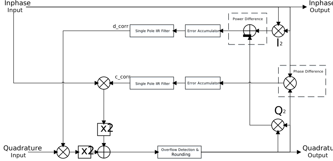
Figure 370: IQ Imbalance Fixer Block Diagram.

Design

The full resolution is maintained for the loop error accumulation. The accumulated results have zero padding applied to the LSBs to increase the underlying data width from \(2 \times \text{data_width}\) to accumulator_precision. Then discarding log2_averaging_length least significant bits from the accumulation through truncation results in an average power and phase difference with accumulator_precision data_width. Note, it is important that the negation in the phase difference IIR filter is performed after the truncation because truncation does not round symmetrically around zero.

The phase IIR filter corrects phases over a positive or negative range and so is initialised to zero. The power IIR filter corrects over a solely positive range, so it is initialised to half the maximum positive value (just the \(MSb-1\) set). Values above/below this point will apply a gain/attenuation respectively. This means when calculating the corrected Q values, \(2 \times D\) is actually used, to provide zero gain when the IIR filter is at its initial state, and \(2 \times C\) is used aligning the phase dynamic range with the power product.

The IIR filters have a pole on the unit circle and have gain of \(2^{\text{-neg_log2_loop_gain}}\), achieved by discarding neg_log2_loop_gain least significant bits from the average power and phase differences through truncation. Note, the bits are discarded on the filter input but the IIR filters themselves operate with accumulator_precision bits of precision.

Once a corrected Q value is calculated, overflow detection checks for overflow in the upper 4 bits. If a positive/negative overflow is detected, a saturated positive/negative result is returned. Otherwise, the upper 3 bits are discarded and the lower bits are returned. Finally, the result is rounded down to the original input width using half-even rounding.

On initialisation, \(2^{\text{log2_averaging_length}}\) samples need to be processed without applying gain/offset corrections. From this point onwards, corrected samples will be output with the correction changing every \(2^{\text{log2_averaging_length}}\) samples. If a flush or discontinuity opcode is received the loop error accumulation restarts, so the next correction update is again \(2^{\text{log2_averaging_length}}\) samples away, but the calculated corrections are retained and continue to be applied in the meantime.

Interface

Opcode Handling

• Samples

  • Apply the previously calculated power and phase corrections to the received Quadrature samples.

  • Saturate the corrected Quadrature samples if they overflow, and then round to the output width.

  • Send the received In-phase and calculated Quadrature samples to the output port.

  • Update the calculated power and phase correction algorithm with the output samples.

• Time

  • Forward to output port.

• Sample_Interval

  • Forward to output port.

• Flush

  • Clear the loop error accumulators, retaining the calculated power and phase corrections.

  • Forward to output port.

• Discontinuity

  • Clear the loop error accumulators, retaining the calculated power and phase corrections.

  • Forward to output port.

• Metadata

  • Forward to output port.

Properties

• enable: Enable/bypass control.

  • Type: bool

  • Access:

    • Parameter: False

    • Writable: True

    • Initial: False

    • Volatile: False

  • Default value: true

• update: Update the calculated amplitude and phase errors or hold previous.

  • Type: bool

  • Access:

    • Parameter: False

    • Writable: True

    • Initial: False

    • Volatile: False

  • Default value: true

• neg_log2_loop_gain: Loop gain control, where the value is 2^(-n). Must be less than or equal to 31.

  • Type: uchar

  • Access:

    • Parameter: False

    • Writable: True

    • Initial: False

    • Volatile: False

  • Default value: 5

• log2_averaging_length: Update interval control, where 2^(n) samples define the averaging length. Must be greater than or equal to 5 and less than or equal to 31.

  • Type: uchar

  • Access:

    • Parameter: False

    • Writable: True

    • Initial: False

    • Volatile: False

  • Default value: 9

• accumulator_precision: Number of most significant bits of precision preserved from the accumulator.

  • Type: uchar

  • Access:

    • Parameter: True

    • Writable: False

    • Initial: False

    • Volatile: False

  • Default value: 34

Ports

Inputs:

• input: Primary input samples port.

  • Protocol: complex_short_timed_sample-prot

  • Optional: False

Outputs:

• output: Primary output samples port.

  • Protocol: complex_short_timed_sample-prot

  • Optional: False

Implementations

• iq_imbalance_fixer_xs (HDL)

  An HDL implementation of the IQ Imbalance Fixer

• iq_imbalance_fixer_xs (RCC)

  An RCC implementation of the IQ Imbalance Fixer

Example Application

<?xml version="1.0"?>
<application done="file_write">
  <instance component="ocpi.core.file_read" connect="iq_imbalance_fixer_xs">
    <property name="filename" value="input.bin"/>
  </instance>
  <instance component="ocpi.comp.sdr.dsp.iq_imbalance_fixer_xs" connect="file_write">
    <property name="enable" value="true"/>
    <property name="update" value="true"/>
    <property name="log2_averaging_length" value="11"/>
    <property name="neg_log2_loop_gain" value="5"/>
    <property name="accumulator_precision" value="34"/>
  </instance>
  <instance component="ocpi.core.file_write">
    <property name="filename" value="output.bin"/>
  </instance>
</application>

Dependencies

• HDL dependencies:

  • The dependencies to other elements in OpenCPI are:

    • IQ Imbalance Corrector primitive

    • Protocol interface FIFO primitive v2

  • There is also a dependency on:

    • ieee.std_logic_1164

    • ieee.numeric_std

    • ieee.math_real

• RCC OpenCPI dependencies:

  • components/math/common/scale_round.hh

Limitations

• The HDL and RCC workers are not necessarily functionally interchangeable — their outputs differ, so an HDL worker cannot be swapped for an RCC one (or vice versa) expecting identical behaviour. The HDL error-feedback path is pipelined, so each power and phase correction update is applied several samples after the output that produced it, whereas the RCC worker applies corrections without this delay.

• The maximum update interval control is tested up to 31 since HDL timing performance is negatively impacted with higher values. Also, it must be set such that the averaging length is greater than the internal HDL pipeline length that calculates power and phase correction values. Therefore \(5 \leq\) log2_averaging_length \(\leq 31\).

• The maximum loop gain control (i.e the neg_log2_loop_gain property) is 31, limiting the loop gain to \(2^{-31}\). This is to limit the widths of internal signals in the HDL worker, to improve resource usage and timing performance.

Testing

A number of tests have been performed on this component. They are all a variation of the same test, but use different property values, different input sample ranges, and different message combinations.

Model Validation

The Python implementation of the component has been tested via a pytest. As part of this pytest an input file is generated consisting of a waveform with tones at 5 Hz, 13 Hz, and 27 Hz. A spectral image is created by both adding a different gain to I and Q rails, as well as adding an additional 10 degrees of phase to the sine portion of the complex signal. This results in the addition of spectral image tones at -5 Hz, -13 Hz, and -27 Hz which are shown as the blue input spikes in the Input Spectral Image graph in Figure 371:.

The complex waveform is scaled to fixed-point signed 16-bit integers, with a maximum amplitude of 32000 to avoid roll-over. The pytest checks that the 3 highest peaks in the output (in the frequency domain) corresponds to the generated tones 5 Hz, 13 Hz, and 27 Hz. The pytest then checks that the next 3 highest peaks are at a sufficiently low level, therefore testing that the negative frequency spikes (spectral images) have been attenuated. The Power spectrum graph in Figure 371: shows the balanced output which only contains the 5 Hz, 13 Hz, and 27 Hz tones.

Note: The verification of the output data is performed only on the second half of the output, which represents the steady state of the component.

Finally the input and output data are translated to the frequency domain, where a FFT is performed, and then power measurements are observed to check that the expected positive frequency output tones are present. The Power Difference graph in Figure 371: shows that the negative spectral image tones have been attenuated by at least 65 dB in comparison to the original input data.

The test results may be viewed in Figure 371: below:

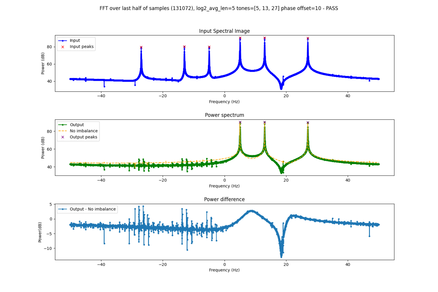
Figure 371: Test Results

Component Testing

Tested platforms: None

Component testing not completed.