Non-Data-Aided Adaptive Equaliser (nda_adaptive_equaliser_xs)

Non-data-aided (blind) adaptive equaliser using a feed-forward architecture.

Design

Adaptive equalisers are a specialised class of filters designed to compensate for time-varying, complex-valued distortions introduced by a communication channel. They are commonly employed to mitigate effects such as echo, inter-symbol interference (ISI), fading, amplitude distortion, and phase rotation.

Architecturally, adaptive equalisers are typically realised as either finite impulse response (FIR) or infinite impulse response (IIR) structures. Two widely used forms are:

• Feed-forward equalisers (FFE) - Use only past input samples and offer relatively low computational complexity.

• Decision-feedback equalisers (DFE) - Include a feedback path driven by symbol decisions at the output, improving ISI performance at the cost of additional complexity.

Unlike fixed filters, adaptive equalisers use complex tap coefficients that are continuously updated according to an adaptation algorithm.

Adaptation algorithms generally fall into three categories:

• Data-aided - Use known training sequences (preambles or pilot symbols) to estimate the channel response.

• Non-data-aided (blind): Use only the received samples, without relying on any transmitted reference symbols.

• Decision-directed: Use demodulator decisions once the equaliser has partially converged, refining the tap estimates.

This component implements the non-data-aided approach, enabling operation on arbitrary input streams without requiring training sequences.

It employs a feed-forward architecture. Channel compensation is performed using complex-valued tap coefficients, which correct both amplitude and phase distortions introduced by the channel.

It supports two algorithms for tap adaptation, CMA and MMA, as described in the Channel Estimation section. Being a non-data-aided implementation, tap updates are performed on every incoming sample. Providing initial tap values based on prior channel estimates can significantly reduce convergence time; otherwise, the worker defaults to \([(1+0j), 0, 0, ...]\).

An example block diagram illustrating a feed-forward blind equaliser and its tap calculation is shown in Figure 373:.

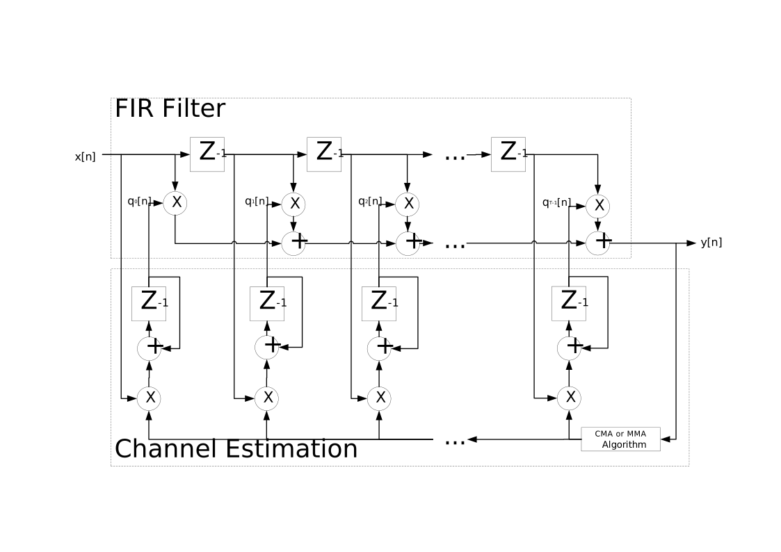
Figure 373: Example implementation of a feed-forward adaptive equaliser.

Channel Estimation

Channel estimation determines the values of the equaliser’s tap coefficients. Various algorithms can be used to compute an error signal, which is then applied to update the taps. This component supports two algorithms: Constant Modulus Algorithm (CMA) and Multi-Modulus Algorithm (MMA).

The equalised output of the component is computed as:

(78)\[y[n] = q^T[n] x[n]\]

where

• \(q^T[n]\) is the N-tap coefficient vector at sample \(n\)

• \(x[n]\) is the input vector at sample \(n\)

• \(^T\) denotes the transpose operation

Constant Modulus Algorithm

The Constant Modulus Algorithm (CMA) is used to adjust signals toward a constant modulus power envelope (i.e., onto the unit circle) while also correcting minor inter-symbol interference (ISI). CMA does not provide phase correction and attempts to force all input samples onto a single radius in the IQ plane.

This makes CMA particularly well suited for signals with a single amplitude level, such as 4-QAM, QPSK, or 2-FSK.

The error calculation is illustrated in Figure 374:, and the tap update is defined by:

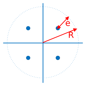
Figure 374: Error calculation between the input sample magnitude and the unit-modulus circle.

(79)\[q^*[n+1] = q^*[n] + \mu\, y^*[n] \left( R^2 - |y[n]|^2 \right) x[n]\]

where

• \(^*\) denotes complex conjugation

• \(\mu\) is the step size

• \(R\) is the unit modulus (radius of the target circle)

This can alternatively be expressed in non-conjugate form as:

(80)\[q[n+1] = q[n] + \mu\, y[n] \left( R^2 - |y[n]|^2 \right) x^*[n]\]

Key points about CMA:

• Corrects magnitude but does not correct phase. Samples already on the unit circle will produce no further error.

• Best suited for single-amplitude constellations. CMA is not recommended for multi-level QAM (e.g., 16-QAM or higher).

The effect of CMA on an attenuated input signal is illustrated in Figure 375:.

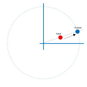
Figure 375: Correction of an attenuated input signal using CMA and the corresponding error feedback loop.

Multi-Modulus Algorithm

The Multi-Modulus Algorithm (MMA) adjusts the I (real) and Q (imaginary) components of the signal separately toward the unit modulus. This provides an advantage over CMA, as MMA can correct for rotation in the IQ plane in addition to magnitude distortions.

For an order-4 constellation, the error calculation is illustrated in Figure 376:, and the tap update is defined by:

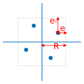
Figure 376: Error calculation for MMA, showing correction of I and Q components toward the unit modulus.

(81)\[q^{*}[n+1] = q^{*}[n] + \mu \left( y_{I}[n] \left(R^2 - y_{I}^2[n]\right) + j y_{Q}[n] \left(R^2 - y_{Q}^2[n]\right) \right)^{*} x[n]\]

where

• \(y_I[n]\) is the real part of the equalised output

• \(y_Q[n]\) is the imaginary part

• \(R\) is the unit modulus on both axes

• \(^*\) denotes complex conjugation

This can alternatively be expressed in non-conjugate form as:

(82)\[q[n+1] = q[n] + \mu \left( y_{I}[n] \left(R^2 - y_{I}^2[n]\right) + j y_{Q}[n] \left(R^2 - y_{Q}^2[n]\right) \right) x^{*}[n]\]

The effect of MMA on an attenuated order-4 input signal is shown in Figure 377:.

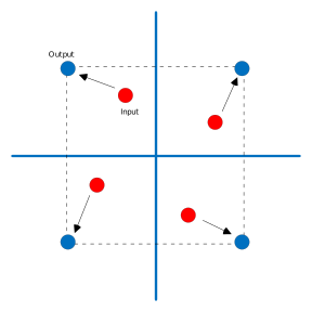
Figure 377: Correction of an attenuated order-4 input signal using MMA and the corresponding error feedback loop.

Order 16 and Order 64 Mapping

The MMA algorithm is designed to operate on order-4 constellations, where each quadrant contains a single constellation point. For higher-order QAM signals (e.g., 16-QAM or 64-QAM) where points appear at amplitudes such as R, 3R, 5R, etc., the points must be mapped to an equivalent order-4 representation. This is accomplished by shifting the origin into the quadrant containing each point.

• 16-QAM - Can be decomposed into 4 order-4 constellations, one per quadrant

• 64-QAM - Can be decomposed into 16 order-4 constellations by first mapping each quadrant as an order-16 constellation and then applying the order-16 to order-4 transformation

The steps for mapping a specific point (highlighted in red) are illustrated in Figure 378::

• The point lies in the top-right quadrant of the original constellation. The origin is shifted to the centre of this quadrant, yielding an order-16 constellation.

• Within the order-16 constellation, the point is again located in the top-right quadrant, so the origin is shifted to that quadrant.

• The resulting order-4 constellation places the point in the bottom-left quadrant of the mapped order-4 region.

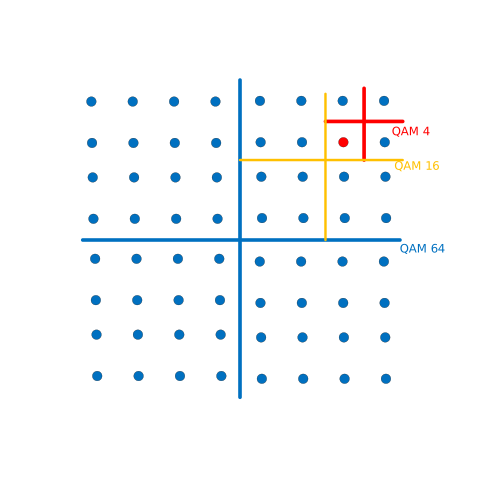
Figure 378: Example of mapping a point from a 64-QAM constellation into an order-4 constellation for MMA processing.

Note: Although this quadrant-mapping technique can theoretically be applied to CMA, this implementation restricts CMA to order 4, as it is not suitable for higher-order QAM constellations.

RCC and HDL Behaviour Characterisation

This section highlights the differences in performance between the HDL and RCC implementations of the adaptive equaliser.

The HDL implementation is pipelined, which introduces differences in behaviour compared to the non-pipelined RCC design. The plots and examples in this section illustrate these differences and help visualise the performance characteristics of each implementation.

Error Vector Magnitude

Error Vector Magnitude (EVM) is a widely used metric for quantifying the performance of a digital receiver. It measures the deviation of received constellation points from their ideal positions.

Distortions in the received signal cause points to drift away from their ideal locations, increasing the EVM and indicating degraded performance.

In this characterisation, EVM is computed as follows:

1. Calculate the root mean square (RMS) of the error vector between the transmitted and received signals:

(83)\[Error_{rms} = \sqrt{\mathrm{mean}\left(|TxSignal - RxSignal|^2\right)}\]

2. Calculate the RMS amplitude of the transmitted signal:

(84)\[Tx_{rms} = \sqrt{\mathrm{mean}\left(|TxSignal|^2\right)}\]

3. Compute the normalized EVM in dB:

(85)\[EVM\,[\mathrm{dB}] = 20 \cdot \log_{10}\frac{Error_{rms}}{Tx_{rms}}\]

EVM Plots

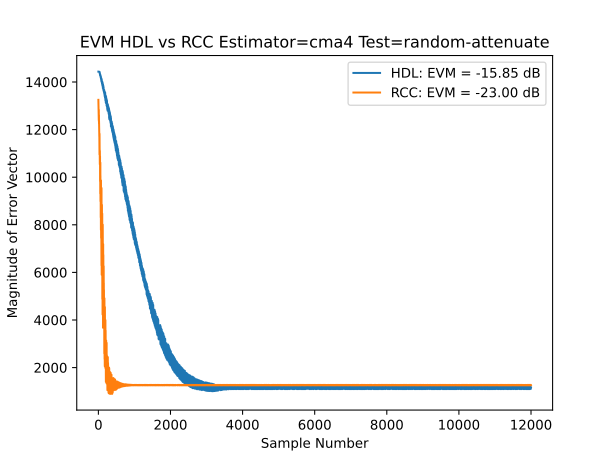
The plots below illustrate the behaviour of the RCC (non-pipelined) design compared to the HDL (pipelined) design for input sample tests. A random attenuation effect was applied to simulate realistic channel distortions. This linear attenuation allows a clear comparison between the two implementations.

Each plot shows the magnitude of the error vector per sample, indicating how far each equalised sample deviates from its ideal constellation point, rather than showing a mean over all samples. The overall Error Vector Magnitude (EVM) for both RCC and HDL designs is also depicted.

These results were generated using an attenuated input signal for four different estimators with three taps. In the plots:

• The y-axis represents the magnitude of the error vector

• The x-axis represents the number of processed samples

• Maximum error vector magnitude is higher for lower-order constellations and decreases for higher orders, due to the smaller maximum possible deviation

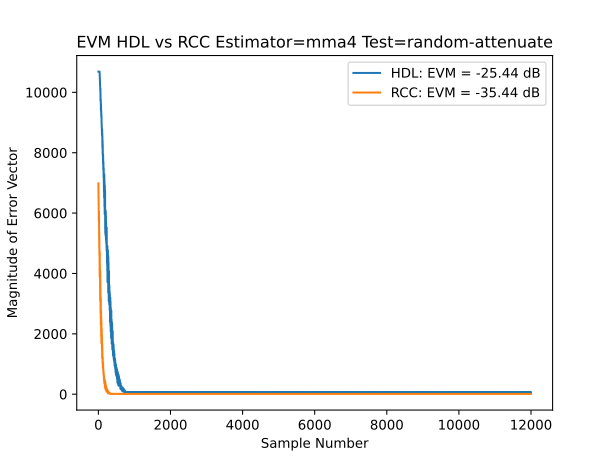
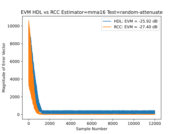
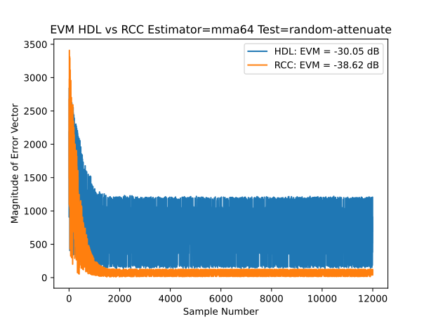
In the final plot, larger variations in error magnitude are observed after the equaliser settles. This is due to quantisation errors in the HDL implementation resulting from its fixed bit-width arithmetic.

As the number of processed samples increases, the error magnitude decreases, indicating that the taps are converging to correct the output. In general, the HDL model requires more samples to converge than the RCC model, which is expected due to the pipelined architecture.

The HDL implementation is intended for higher sample rates than the RCC worker, allowing the equalised output to converge faster in real-time conditions.

To illustrate the effect of sampling rate, the plot below compares error vectors for HDL and RCC operating over the same period, but with different sampling rates:

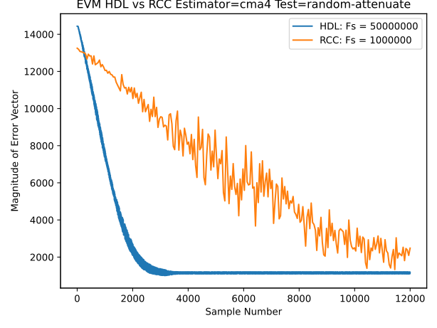
Here, the HDL is running at 50 Msps, while the RCC operates at 1 Msps. The higher HDL sampling rate allows faster convergence of the equaliser.

When using a larger number of taps (e.g., 21 taps) at the same sample rate, the performance of the HDL and RCC implementations becomes nearly identical, as shown below:

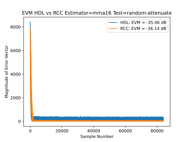
This plot demonstrates that, with sufficient taps, the HDL converges to the equalised values similarly to the RCC implementation.

References

• 19. Abrar, R. A. Axford Jr, “Sliced Multi-modulus Blind Equalization Algorithm”, ETRI Journal, vol. 27, no. 3, pp. 257-266, 2005.

• 10. Yang, “Multi-modulus Algorithms for Blind Equalization”, University of British Columbia, 1997.

• 7. Giunta, F. Benedetto, “A Signal Processing Algorithm for Multi-Constant Modulus Equalization”, 2013 36th International Conference on Telecommunications and Signal Processing (TSP), pp 52-56, 2013.

• K Banovic, Kevin, “Blind adaptive equalization for QAM signals: New algorithms and FPGA implementation.” Electronic Theses and Dissertations - 1312, 2006.

Interface

<?xml version="1.0"?>
<componentspec>
  <property name="estimator" type="enum" parameter="true" enums="cma,mma" default="cma"
    description="Estimation algorithm to use within this component"/>
  <property name="order" type="uchar" initial="true" default="4" description="Order of QAM signal (4, 16, 64)"/>
  <property name="number_of_taps" type="uchar" parameter="true" default="3" description="Number of complex taps."/>
  <property name="unit_modulus" type="short" initial="true" default="23170"
    description="Unit Modulus for use in error estimation, as a Q1.15 (Note: Only positive values are allowed)"/>
  <property name="step_size" type="ushort" initial="true" default="1536"
    description="Error step size (:math:`\mu`), as a UQ1.15 value."/>
  <property name="taps_real" type="short" arraylength="number_of_taps" initial="true" default="32767"
    description="Initial real tap values as Q1.15. Defaults to 1.0 for the first tap and 0 for the rest."/>
  <property name="taps_imag" type="short" arraylength="number_of_taps" initial="true" default="0"
    description="Initial imaginary tap values as Q1.15. Defaults to all zeros."/>
  <port name="input" producer="false" protocol="complex_short_timed_sample-prot"/>
  <port name="output" producer="true" protocol="complex_short_timed_sample-prot"/>
</componentspec>

Ports

Inputs:

• input: Primary input samples port.

  • Protocol: complex_short_timed_sample-prot

  • Optional: False

Outputs:

• output: Primary output samples port.

  • Protocol: complex_short_timed_sample-prot

  • Optional: False

Opcode Handling

The component handles opcodes as follows:

• Sample opcode - Provides data to the processing path as described in the Design section.

• Flush opcode - Feeds number_of_taps zero-valued samples into the equaliser and emits the resulting output as its own message, then forwards the flush opcode.

• Discontinuity opcode - The sample history is cleared so that old samples do not contribute to subsequent outputs, but the adapted tap coefficients (the learnt channel estimate) are retained. The discontinuity opcode is then forwarded to the output.

• All other opcodes - Passed through the component without modification.

Properties

• estimator: Estimation algorithm to use within this component.

  • Type: enum

    • Allowed values: ['cma', 'mma']

  • Access:

    • Parameter: True

    • Writable: False

    • Initial: False

    • Volatile: False

  • Default value: cma

• order: Order of QAM signal (4, 16, 64).

  • Type: uchar

  • Access:

    • Parameter: False

    • Writable: False

    • Initial: True

    • Volatile: False

  • Default value: 4

• number_of_taps: Number of complex taps.

  • Type: uchar

  • Access:

    • Parameter: True

    • Writable: False

    • Initial: False

    • Volatile: False

  • Default value: 3

• unit_modulus: Unit Modulus for use in error estimation, as a Q1.15 (Note: Only positive values are allowed). For CMA, this is the complex modulus defining the radius of the circle onto which the constellation points are projected. For MMA, this is the magnitude of points along the I and Q axes used to adjust each component separately.

  • Type: short

  • Access:

    • Parameter: False

    • Writable: False

    • Initial: True

    • Volatile: False

  • Default value: 23170

• step_size: Error step size (\(\mu\)), as a UQ1.15 value.

  • Type: ushort

  • Access:

    • Parameter: False

    • Writable: False

    • Initial: True

    • Volatile: False

  • Default value: 1536

• taps_real: Initial real tap values as Q1.15. Defaults to 1.0 for the first tap and 0 for the rest.

  • Type: short

    • Array dimensions: ['number_of_taps']

  • Access:

    • Parameter: False

    • Writable: False

    • Initial: True

    • Volatile: False

  • Default value: 32767

• taps_imag: Initial imaginary tap values as Q1.15. Defaults to all zeros.

  • Type: short

    • Array dimensions: ['number_of_taps']

  • Access:

    • Parameter: False

    • Writable: False

    • Initial: True

    • Volatile: False

  • Default value: 0

Implementations

• nda_adaptive_equaliser_xs (HDL)

• nda_adaptive_equaliser_xs (RCC)

Example Application

<?xml version="1.0"?>
<application done="file_write">
  <instance component="ocpi.core.file_read" connect="nda_adaptive_equaliser_xs">
    <property name="filename" value="input.bin"/>
  </instance>
  <instance component="ocpi.comp.sdr.dsp.nda_adaptive_equaliser_xs" connect="file_write">
    <property name="estimator" value="cma"/>
    <property name="order" value="4"/>
    <property name="number_of_taps" value="13"/>
    <property name="unit_modulus" value="23170"/>
    <property name="step_size" value="1536"/>
    <property name="taps_real" valuefile="real.dat"/>
    <property name="taps_imag" valuefile="imag.dat"/>
  </instance>
  <instance component="ocpi.core.file_write">
    <property name="filename" value="output.bin"/>
  </instance>
</application>

Dependencies

The dependencies to other elements in OpenCPI are:

• HDL OpenCPI dependencies:

  • Adaptive equaliser primitive

  • Protocol interface fifo primitive v2

• RCC OpenCPI dependencies:

  • components/dsp/common/fir/fir_core.hh

There is also a dependency on:

• HDL specific dependencies:

  • ieee.std_logic_1164

  • ieee.numeric_std

  • ieee.math_real

• RCC specific dependencies:

  • cmath

  • utility

  • vector

Limitations

Limitations of nda_adaptive_equaliser_xs are:

• The HDL and RCC workers are not necessarily functionally interchangeable — their outputs differ, so an HDL worker cannot be swapped for an RCC one (or vice versa) expecting identical behaviour. The HDL error-feedback path is pipelined, so each tap update is applied several samples after the output that produced it, and it uses reduced-precision arithmetic to save FPGA resources.

• Both CMA and MMA estimators are sensitive to the choice of step size. A step size that is too large can cause the estimator to become unstable and produce invalid output. A step size that is too small slows convergence, reducing the equaliser’s ability to respond to changes in the signal

• Both CMA and MMA algorithms adjust slowly, making them better suited for steady-state signal distortions rather than rapid bursts of interference or fast-changing channel conditions

• CMA corrects magnitude, not phase, and only supports order-4 constellations; higher-order QAM is not suitable for CMA.

Testing

Tested platforms: None

Component testing not completed.