Polyphase Clock Synchroniser (polyphase_clock_synchroniser_xc)

Introduction

A symbol clock synchroniser produces symbols from a stream of samples. The most basic clock synchroniser works by picking a single sample out of the stream at the correct symbol rate (this ratio is known as the samples per symbol, or SPS). The problem with this simple approach is knowing whether the chosen sample is at the optimal location within the sample stream. This problem is shown in Figure 301: below. The orange line shows the best sampling location, however if the stream was just down-sampled by SPS then you might end up actually sampling at the grey location. If the signal to noise ratio (SNR) is good, then this might be acceptable. However as the SNR drops, the chances of getting a bit error when decoding in this bad location increases.

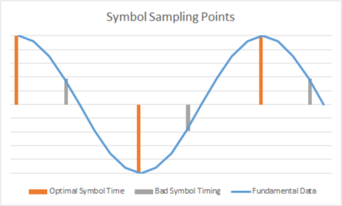
Figure 301: Symbol Sampling Points

In order to allow the selection of the best sampling point there needs to be some method of determining where the peaks and the zeros are in the data. At the most basic this can be achieved through a peak detector running over the SPS number of points. However, this is only a useful method if there are a high number of samples per symbol. If, however, there are only a few samples per symbol, it is necessary to instead interpolate first to allow this selection of an optimum point.

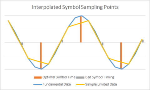
Figure 302: Interpolated Symbol Sampling Points

The interpolation allows the selection of the optimum points, where the number of samples per symbol is too low to rely on a direct down-sampling. The interpolation also is preferable to down-sampling because the additional low pass filter used within the interpolation filter can be shaped to the samples per symbol which will provide a processing gain compared to a direct down-sample.

Design

The polyphase symbol clock synchroniser attempts to recover symbol timing for an incoming data stream. Symbols are output from the component.

The symbol synchronisation is undertaken through the stages shown in Figure 303: below. This block is intended to detect and synchronise to a symbol stream for simple zero crossing modulation schemes (i.e. FSK, PSK).

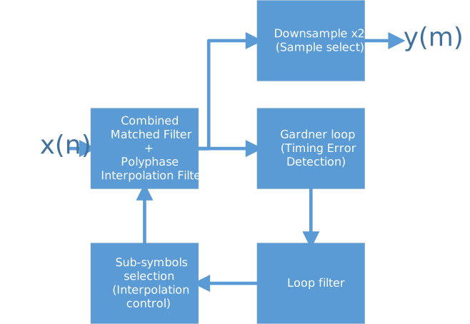
Figure 303: Synchronisation Stages

• \(x(n)\) defines the incoming (unsynchronised) symbol stream (at 2x regenerated sampling period)

• \(y(m)\) defines the outgoing symbol data (at regenerated sampling period)

• \(e(m)\) defines the outgoing calculated symbol error (at 2x regenerated sampling period)

Each of these stages are detailed below.

The implementation handles bandwidth limited signals (i.e. that are known to have 2 incoming samples for a single outgoing symbol).

The timing error detection uses a Gardner zero crossing detection method; this is suited to lower orders of modulation.

Notes

• The incoming data and the polyphase interpolation filter are assumed to be run at 2x the desired output symbol rate. This is to prevent ambiguity if the previous decimating filter / ADC was badly matched to the filter.

• The down sample by 2 is a simple 1 in 2 sample selection (i.e. no low pass filter present) - this is acceptable as every other sample should be the zero crossing point (as needed for the Gardner loop).

• Interpolation filter selection and loop filter should be free-running to allow for n-FSK functionality (i.e. if no zero crossing is detected then the error is ignored as opposed to being considered maximal).

• The selection of sub symbol may undergo a step change due to clock synchronisation. This is limited to only a single step per loop cycle.

• For FSK modulation, matched filtering does not really perform as desired (zero crossing RRC can lead to the need for quadrature modulation methods). Therefore, a Gaussian transmit pulse shaping will show better performance in a real only demodulator.

References

1. Symbol Synchronization for SDR Using a Polyphase Filterbank Based on an FPGA P. Fiala and R. Linhart (2015)

2. Multirate Digital Filters for Symbol Timing Synchronization in Software Defined Radios F. Harris, M. Rice (2001)

3. Samples to Digital Symbols [GRCON2017] A Walls (2017)

Combined Matching and Polyphase Interpolation Filter (Real)

The interpolation structure used within this component consists of a single multiply-accumulate (MAC) unit. This provides a resource efficient method, but limits the maximum possible throughput. As up to 2 polyphase branches might be calculated (if sample stuffing is occurring), the input throughput should be low enough that \(2 \times \texttt{taps_per_branch}\) multiply-accumulate calculations can occur for each input sample.

The tap values and the number of taps to use is run-time settable, however a hard limit is defined as well to limit the amount of memory required.

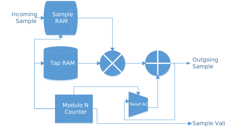
Figure 304: Polyphase Interpolation Filter

Design

New samples are inserted within the sample RAM, which acts as a simple circular buffer of the last N samples (where N is equal to the FIR tap count divided by the number of polyphase branches).

When a new sample is inserted…

1. The relevant polyphase branch b0 tap is multiplied by the new sample.

2. The modulo counter then jumps to the next tap for that branch (a jump of the up sampling ratio), and then multiplies with the z-1 incoming sample.

3. The modulo counter continues until all the taps for that branch have been through the MAC. The output is then registered and the output Sample Valid line set High.

4. The accumulator is then internally reset, awaiting the next incoming sample.

Gardner loop detector

The Timing Error detector implemented is a Gardner zero crossing detector. This works by comparing the zero crossing location against the difference between two symbols. Therefore an incoming sample rate of at least twice that of the output symbol rate is required.

The Gardner loop has the form: Error = Prompt x (Late - Early) This is shown within Figure 305: with the \(n_3\) value being used for the Prompt variable. However, as the data stream should be centred around zero, if shifted by one position, i.e. using \(n_3\), \(n_4\) and \(n_5\), the timing error detector would produce an error with the opposite sign.

As can be seen in Figure 306:, under a signal varying in the range (-1, 1) the error limits are also bounded to the same region (with the greatest error occurring at 45 degrees lag/lead - as there are 4 samples per cycle).

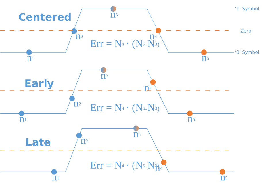
Figure 305: Symbol location for Early/Late samples

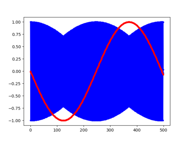
Figure 306: Error Variation with varying sample phase

Notes

1. A Gardner loop is sensitive to any DC bias upon the incoming samples (caused by the non-differentiated term).

2. If there is no hard decision on the incoming samples (i.e. there is a magnitude as opposed to being exactly -1 or 1), then additional timing errors can be introduced by a run of the same symbol. To get around this a sign comparison of all three terms is used to ensure only zero crossings are used.

3. If the input energy is varying with time (likely with an FM phase differential discriminator), then there should be an AGC block, stabilising this data. Without that, the output from the loop will not have the same proportional gain as is expected by the loop filter/PLL.

4. The coarse estimation of the number of samples per symbol is not part of this element, only the fine correction undertaken naturally through the timing estimation.

Loop Filter

The realistic output of the timing error detector is not a smooth curve as defined above, but instead a choppy set of values (caused by sampling clock errors, and slight frequency misalignment). As such a Phase Locked Loop (PLL) loop filter is desired to help smooth the variation seen. This should be a second order PI (Proportional-Integral) loop filter, as there is a need for phase recovery (sub sample alignment using the interpolator), as well as frequency recovery (clock misalignment, leading to drift, using the interpolator, and incoming sample stuff/skip).

The loop filter has the following equations:

\[E_i = (\texttt{ted} \times K_i) + E_i\]

\[Err = E_i + (\texttt{ted} \times K_p)\]

• \(\texttt{ted}\) is the timing error detector output, (multiplied by any scaling required)

• \(K_p\) is the proportional filter constant

• \(K_i\) is the integrator filter constant

• \(E_i\) is the integral error value

• \(Err\) is the resultant error value

This is shown below as the start of the tap selection logic.

Sample and Tap Selection

The tap and sample selection is shown in Figure 307: below. The output of the Timing Error Detector is filtered, then accumulated. This accumulated value provides the phase error. A wrapping detector allows for small frequency adjustment.

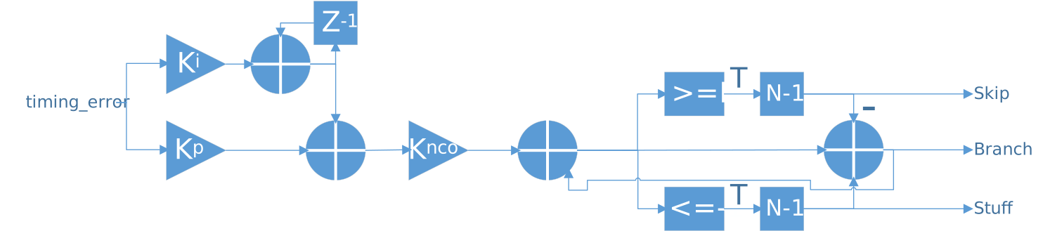
Figure 307: Sample and Tap Selection

The Gardner timing error detector produces an output which has a magnitude related to the distance of the sample away from the zero crossing. As this value is used to correct the sample timing error, this value is negated.

The output from this timing error could lead to the zero crossing and actual usable samples being the wrong way round. To help detect this, the output symbol forwarded is the symbol with the highest magnitude of the two.

This symbol selection method can handle phase offsets from any sampling phase and small frequency errors (i.e. less than 100 ppm). However, this will not correct for a coarse frequency error, without an additional output sample skip/stuff mechanism.

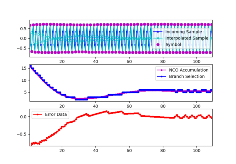
Figure 308: Phase correction with small initial symbol phase offset

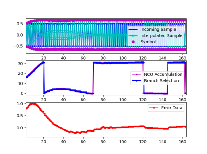
Figure 309: Phase correction with large initial symbol offset

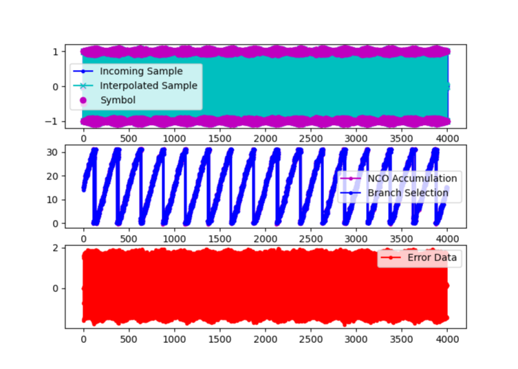
Figure 310: Frequency Correction (note ever changing branch)

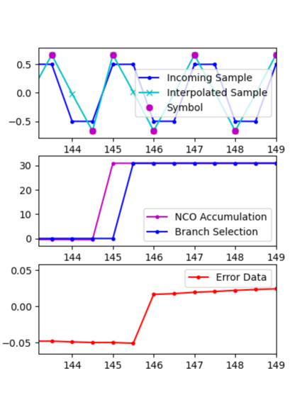
Figure 311: Symbol Skipping (145)

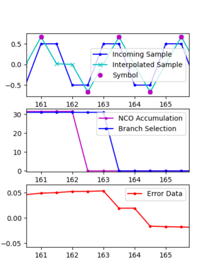
Figure 312: Symbol Stuffing (162)

As the incoming data stream contains complex data, there are 2 zero crossing detectors (one for In-phase, and another for Quadrature).

Interface

<?xml version="1.0"?>
<componentspec>
  <property name="rounding_type" type="enum" parameter="true" enums="truncate,half_up,half_even" default="half_even"
    description="Selects the sample rounding type"/>
  <property name="max_number_of_taps" type="ushort" parameter="true" default="64"
    description="Defines the maximum number of taps across all interpolation branches"/>
  <property name="interpolation_factor" type="uchar" initial="true" writable="false" default="8"
    description="Defines the number of branches that can be used for interpolation"/>
  <property name="number_of_taps" type="ushort" initial="true" writable="false" default="max_number_of_taps"
    description="Number of taps that are actually being used per interpolation branch"/>
  <!-- Note: This taps property is short, not char.  When set to char, build and
             test generation succeed, but tests are not run as no "acceptable
             implementations" are found. -->
  <!-- LINT EXCEPTION: xml_012: 2:
       Cannot set default as size varies with parameter values. -->
  <property name="taps" type="short" arraylength="max_number_of_taps" writable="true" description="Polyphase interpolation taps"/>
  <property name="loop_coefficients" arraylength="3" type="short" writable="true" default="24,8,8"
    description="Coefficients for the loop filter and NCO"/>
  <port name="input" producer="false" protocol="complex_char_timed_sample-prot"/>
  <port name="output" producer="true" protocol="complex_char_timed_sample-prot"/>
</componentspec>

Ports

Inputs:

• input: Primary input samples port.

  • Protocol: complex_char_timed_sample-prot

  • Optional: False

Outputs:

• output: Primary output samples port.

  • Protocol: complex_char_timed_sample-prot

  • Optional: False

Opcode handling

• Time

  • Incoming: Resynchronises the internal input sample time.

  • Outgoing: This is used in conjunction with the Interpolator tap selection to calculate the outputted symbol time. Note that a change in Sample_Interval might have a delay before the correlating change is made to the outgoing time. Note also that if a Sample_Interval has not been received, the time for the next outputted symbol cannot be calculated, so the time is just passed straight through.

• Sample_Interval

  • Incoming: Value is stored and used in the calculation of the input sample time counter (as detailed above).

  • Outgoing: Sample Interval is set to the incoming sample interval multiplied by 2 (i.e. the data rate is halved).

• Flush

  • Zeros are fed in for a length of taps_per_branch (any produced samples are outputted).

  • Then, the Flush is forwarded to output.

• Discontinuity

  • Forwarded to output.

  • The Sample RAM, Accumulator and Loop filter are reset.

• Metadata

  • Forwarded to output.

• Samples

  • Incoming: Samples are consumed, leading to the internal counter and buffers to step on each sample.

  • Outgoing: Symbols are produced at half the rate of the input data stream (i.e. the data is decimated by 2).

Properties

• rounding_type: Selects the sample rounding type.

  • Type: enum

    • Allowed values: ['truncate', 'half_up', 'half_even']

  • Access:

    • Parameter: True

    • Writable: False

    • Initial: False

    • Volatile: False

  • Default value: half_even

• max_number_of_taps: Defines the maximum number of taps across all interpolation branches.

  • Type: ushort

  • Access:

    • Parameter: True

    • Writable: False

    • Initial: False

    • Volatile: False

  • Default value: 64

• interpolation_factor: Defines the number of branches that can be used for interpolation.

  • Type: uchar

  • Access:

    • Parameter: False

    • Writable: False

    • Initial: True

    • Volatile: False

  • Default value: 8

• number_of_taps: Number of taps that are actually being used per interpolation branch.

  • Type: ushort

  • Access:

    • Parameter: False

    • Writable: False

    • Initial: True

    • Volatile: False

  • Default value: max_number_of_taps

• taps: Polyphase interpolation taps. The actual number of taps required is defined through the taps_per_branch * max_interpolation. Tap values are in the range (-1, 1) and passed as fixed point values in S0.7 format (i.e. 1 sign bit and 7 fractional bits), and can be converted to float by dividing by \(2^7\).

  • Type: short

    • Array dimensions: ['max_number_of_taps']

  • Access:

    • Parameter: False

    • Writable: True

    • Initial: False

    • Volatile: False

  • Default value: None

• loop_coefficients: Coefficients for the loop filter and NCO. Structured as: [\(K_p\), \(K_i\), \(K_{nco}\)]. These are actually fixed point values in S5.2 format (i.e. 1 sign bit, 5 integer bits and 2 fractional bits), and can be converted to float by dividing by \(2^2 = 4\).

  • Type: short

    • Array dimensions: ['3']

  • Access:

    • Parameter: False

    • Writable: True

    • Initial: False

    • Volatile: False

  • Default value: 24,8,8

Rounding Methods

The following round methods are offered:

• truncate: Truncates value towards zero (this will lead to a strong DC bias).

• half_up: Round values away from zero (this will lead to a weak bias towards +/- infinity).

• half_even: Round values towards nearest even - convergent rounding (this will lead to no overall direction of bias).

Implementations

• polyphase_clock_synchroniser_xc (RCC)

  Due to the RCC implementation only processing data on each new incoming message, the internal buffers are stored between runs. As such they are stored within the worker class, as a class variable.

• polyphase_clock_synchroniser_xc (HDL)

Example application

<?xml version="1.0"?>
<application done="file_write">
  <instance component="ocpi.core.file_read" connect="polyphase_clock_synchroniser_xc">
    <property name="filename" value="input.bin"/>
  </instance>
  <instance component="ocpi.comp.sdr.dsp.polyphase_clock_synchroniser_xc" connect="file_write">
    <property name="taps_per_branch" value="5"/>
    <property name="taps" valuefile="taps.dat"/>
    <property name="max_interpolation" value="32"/>
    <property name="max_taps_per_branch" value="5"/>
    <property name="rounding_type" value="half_even"/>
    <property name="loop_coefficients" value="8,4,4"/>
  </instance>
  <instance component="ocpi.core.file_write">
    <property name="filename" value="output.bin"/>
  </instance>
</application>

Dependencies

The dependencies to other elements in OpenCPI are:

• Protocol interface delay primitive v2

• Protocol interface FIFO primitive v2

• Flush inserter primitive v2

• Polyphase FIR Interpolator primitive

• Gardner Timing Error Detector primitive

• components/communication/common/gardner_loop/gardner_loop.hh

• components/dsp/common/polyphase_interpolator/polyphase_interpolator.hh

There is also dependencies on:

• ieee.std_logic_1164

• ieee.numeric_std

• ieee.math_real

Limitations

• The synchroniser is designed to work on discriminated samples (i.e. after a discriminator), as opposed to raw ADC samples.

• Initially the timing error detector is designed for 2 complex samples per symbol (for quadrature data).

• Initially this is designed to handle complex modulation order=2 or 4.

Testing

Component testing not completed.